Linear Transforms Tutorial Sheet, Sheet #4A
Learning Targets
- Understand and produce a graphical representation of a transformation matrix
- Find the transformation matrix for given representations of linear transformations
- Find the null space
- Understand how the relationship between the determinant of a matrix as area scale factor for a linear transformation
Additional Resources
Tutorials
- Linear Algebra Playlist : The same playlist as mentioned last week.
- Rotors and Geometric Algebra : A little extension info video, linking vectors and matrices to how rotors work.
Software
- Freddie’s Matrices Widget : Widget written by our one and only Freddie Page - have an explore and interact to get a good visualisation on how transformations work. Have a go with different types of matrices: Dilations, rotations, shears, reflections, projections and combinations!
- Matlab Documentation : Information on rotational matrices on Matlab. Getting familiar with matlab will be a great advantage.
Problem sheet
Skill Building Questions
Problem 1.
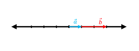
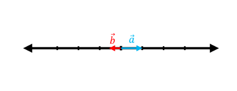
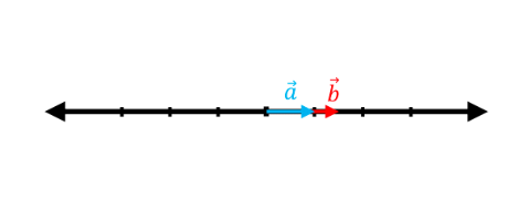
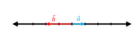
From the following linear transformations, $T:\mathbb{R} \rightarrow \mathbb{R}$ where $T(a) = b$, express $b$ as a function of $a$.
(a)
(b)
(c)
(d)
R Transformation Visualization
To help with intuition when answering these questions, here is a visualization built in Manim. You can play around with it here!
Problem 2.
The following graphs show pairs of vectors where the vector $\vec{a}$ is linearly transformed to $\vec{b}$ by a matrix, $T:\mathbb{R}^2 \rightarrow \mathbb{R}^2$. Considering that these transformations are all pure scalings, find the transformation matrix ($A$) in each case.
(a)
(b)
(c)
(d)
R2 Vector Transformation Visualization
To help with intuition when answering these questions, here is a visualization built in Manim. You can play around with it here!
Problem 3.
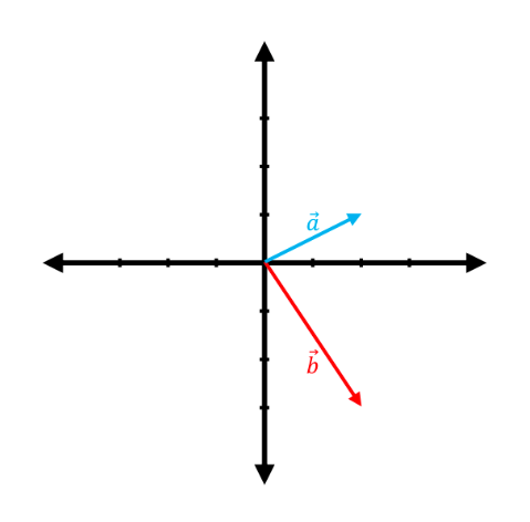
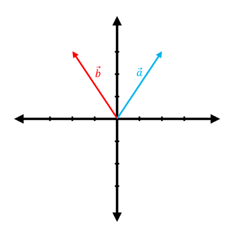
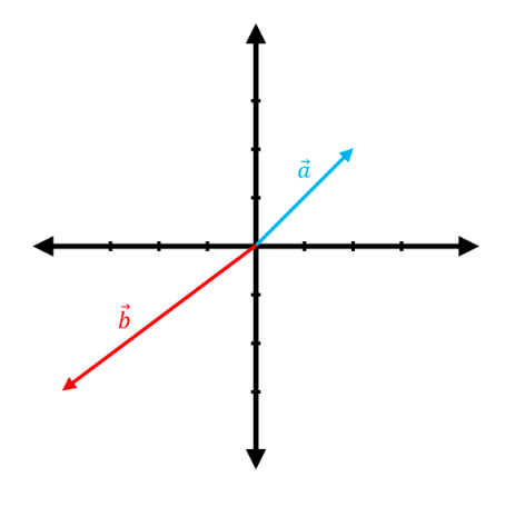
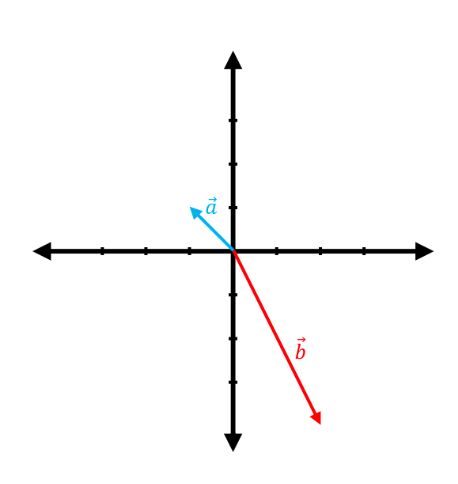
The following graphs show pairs of vectors where the vector $\vec{a}$ is linearly transformed to $\vec{b}$ by a matrix, $T:\mathbb{R}^2 \rightarrow \mathbb{R}^2$. Considering that these transformations are all pure rotations (anti-clockwise from $\hat{i}$ should be assumed for rotations unless otherwise stated, just like for polar coordinates), find the angle $\theta$ and matrix $A$ in each case. $\bigg($NB. $R(\theta)=\begin{pmatrix}\cos{\theta}&-\sin{\theta}\\sin{\theta}&\cos{\theta}\end{pmatrix}\bigg)$
(a)
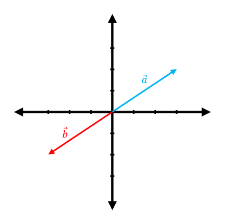
$\Rightarrow{}\quad \cos^{-1}(-1)=180^{\circ}$
(b)
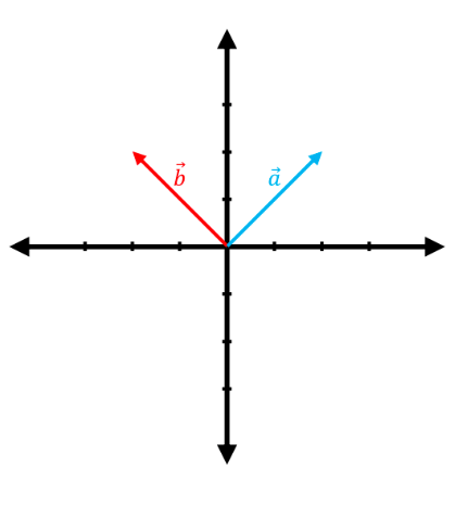
$\Rightarrow{}\quad \sin^{-1}(1)=90^{\circ}$
Problem 4.
From applying a linear transformation, $T:\mathbb{R}^2 \rightarrow \mathbb{R}^2$ where $T(\vec{a}) = \vec{b}$. Find the vector $\vec{b}$ resulting when a clockwise rotation described by $R(\theta)=\begin{pmatrix}\cos{\theta}&\sin{\theta} \\ -\sin{\theta}&\cos{\theta}\end{pmatrix}$ is applied to $\vec{a}$. Sketch the vectors $\vec{a}$ and $\vec{b}$ on a Cartesian axes
(a) $\vec{a}=\begin{pmatrix}2 \newline 2\end{pmatrix}$ and $\theta=60^{\circ}$
$\Rightarrow{}\quad \begin{pmatrix}0.5&0.866\\-0.866&0.5\end{pmatrix} \begin{pmatrix}2\\2\end{pmatrix} = \boxed{ \begin{pmatrix}2.732\\-0.732\end{pmatrix}}$
$\Rightarrow{}\quad$

(b) $\vec{a}=\begin{pmatrix}2 \newline 3\end{pmatrix}$ and $\theta=45^{\circ}$
$\Rightarrow{}\quad \begin{pmatrix}0.7071&0.7071\\-0.7071&0.7071\end{pmatrix} \begin{pmatrix}2\\3\end{pmatrix} = \boxed{ \begin{pmatrix}3.536\\0.7071\end{pmatrix}}$
$\Rightarrow{}\quad$

Problem 5.
From the linear transformations represented in the following figures, obtain the transformation matrix and the change in size (\ie product of change in each dimension, such as area or volume). (NB. The red vector shown is the result of transforming the blue vector.
(a)

(b)

(c)

(d)

(e)

(f)

(g)

(h)

(i)

Note: It’s difficult to see exactly in 3D, but each of the scalings are integers.
R2 and R3 Transformation Visualization
To help with intuition when answering these questions, here is a visualization built in Manim. You can play around with it here!
Problem 6.
For the following linear systems of equations find the null space and the corresponding solution of $x$ and $y$. Sketch the solutions as lines in a Cartesian axes
(a) $\begin{pmatrix}1&1 \\ 2&1\end{pmatrix} \begin{pmatrix}x \\ y\end{pmatrix} = \begin{pmatrix}2 \\ 3\end{pmatrix}$
$\Rightarrow{}\quad \begin{pmatrix}x\\y\end{pmatrix} = A^{-1}b = \begin{pmatrix}-1&1\\2&-1\end{pmatrix} \begin{pmatrix}2\\3\end{pmatrix} \quad\Rightarrow{}\quad \boxed{\begin{pmatrix}x\\y\end{pmatrix} = \begin{pmatrix}1\\1\end{pmatrix}}$

(b) $\begin{pmatrix}2&4\\ 1&3\end{pmatrix} \begin{pmatrix}x\\ y\end{pmatrix} = \begin{pmatrix}6\\ 12\end{pmatrix}$
$\Rightarrow{}\quad \begin{pmatrix}x\\y\end{pmatrix} = A^{-1}b = \begin{pmatrix}3/2&-2\\-1/2&1\end{pmatrix} \begin{pmatrix}6\\12\end{pmatrix}$ $\Rightarrow{}\quad\boxed{\begin{pmatrix}x\\y\end{pmatrix} = \begin{pmatrix}-15\\9\end{pmatrix}}$

Exam Style Questions
Problem 7.
The following figure shows a square in $\mathbb{R}^2$, marked with a circle and cross on its perimeter.

(a) On a single plot, sketch the result of applying the following transformation, A, to the square (including the new locations of the circle and cross) \(A = \begin{bmatrix} 2 \ 0 \\\ 1 \ 1.5\end{bmatrix}\)

(b) Assuming the area of the initial square is 4, what is the area of this region after the transformation?
Extension Questions
Problem 8.
Read the documentation above, found under ‘additional resources’, regarding using Matlab to generate rotational transformation matrices.
(a) Generate a 3D transformation matrix, $\textbf{X}$, for a rotation of 38.4$^{\circ}$ about the x axis, giving your answer to 2 d.p.
Using Matlab:
X = rotx(38.4)
(b) Vector $\textbf{M}$ is mapped to vector $\textbf{T}$ by a rotation of 96.2$^\circ$ about the x axis, followed by a rotation of 112.7$^\circ$
about the y axis. Generate vector $\textbf{T}$ given that:
$\textbf{M} = \begin{pmatrix}
7.2 \newline 42.1 \newline 13.6
\end{pmatrix}$
Using Matlab:
M = [7.2 ; 42.1 ; 13.6]
X = rotx(96.2) * M
T = roty(112.7) * X
Problem 9.
Matrix $\textbf{M}$ is a transformation matrix.
$\textbf{M} = \begin{bmatrix}
2 \ 1 \newline x \ 4
\end{bmatrix}$
(a) When $\textbf{M}$ is applied to a shape of area 3, the resulting area is 21. Find $x$.
$\Rightarrow{} 8-x=7$
$\Rightarrow{} \boxed{x=1}$
(b) Copy and complete the code below, in a new script in Matlab, by adding in the complete transformation matrix. Run the script to visualize the transformation.
%define matrix transformation
M=[];

%define coordinates of original square
x=[-1 1 1 -1 -1];
y=[-1 -1 1 1 -1];

%preallocate transformed coordinate arrays with 0s
X = zeros(1,5);
Y = zeros(1,5);

%loop through coordinates of original square and apply
%the matrix transformation M to each
for i = 1:length(x)
    A = [x(i) ; y(i)];
    A = M * A;


    %define transformed coordinates
    X(i) = A(1,1);
    Y(i) = A(2,1);
end

%plot both the original square and the the transformed shape
hold all
plot(x,y,'LineWidth',3)
plot(X,Y,'LineWidth',3)

%define the axis and legend
axis([-6, 6, -6, 6])
legend('Original','Transformation')
grid on
%define matrix transformation
M=[2 1 ; 1 4];

You now have a crude matrix visualizer, try some different 2D transformation matrices.
Answers
For Printing
Revision Questions
The questions included are optional, but here if you want some extra practice.
- Most matrices questions are all integrated, so the previous and following section will have questions involving transformations. The most important part is getting your head around how it all fits together - I would really recommend Freddie’s widget!